19 Discussion of the Analytical Solution
The piece-wise solutions of Chapter 9 of the
simplest model equations give a lot of approaches for a comprehensive
discussion of the principle behavior of a credit-driven economy. First, we
compare the properly integrated piecewise solution to the IMF 2005 formula.
Exemplary of the GDP at the beginning of the development (![]() ) is:
) is:
![]() (19.1)
(19.1)
![]() (19.2)
(19.2)
We see that the singular IMF 2005 model (18.1) promises a constant growth rate g. The IMF model sets for g the general growth of the capital stock, but in truth, it is of course only the share of invested capital into the GDP. In fact (18.2), it is a combination of exponential and harmonic growth. The hyperbolic functions can be written as exponential function, because it holds
![]() (19.3).
(19.3).
For vanishingly small![]() holds
holds![]() and thus for the
small
and thus for the
small![]() also holds
also holds ![]() . We can
therefore write as an approximation for small arguments
. We can
therefore write as an approximation for small arguments![]() :
:
![]() (19.4)
(19.4)
The argument is
![]() (19.5).
(19.5).
and thus applies to the beginning of the development
![]() (19.6).
(19.6).
Hence we actually start early in the economy with approximately
![]() (19.7)
(19.7)
Analogously, this applies also for![]() , as is easily
verified. At the beginning there is an exponential slope not only of the
capital stock, but also of the GDP. However, not globally but only locally, and
also are there not the same values
, as is easily
verified. At the beginning there is an exponential slope not only of the
capital stock, but also of the GDP. However, not globally but only locally, and
also are there not the same values ![]() for
the slope rates, but
for
the slope rates, but![]() for the GDP and
for the GDP and![]() for the capital
stock. Since in the beginning almost all capital growth gains from direct
investment in GDP, also these values are initially very similar. No wonder then
that singular interpolating models may initially give the impression of a global
scope.
for the capital
stock. Since in the beginning almost all capital growth gains from direct
investment in GDP, also these values are initially very similar. No wonder then
that singular interpolating models may initially give the impression of a global
scope.
Over time, however, the terms![]() and
and![]() develop a very
different behavior as they change to
develop a very
different behavior as they change to![]() and
and![]() terms. Since they
are harmonic functions the argument
terms. Since they
are harmonic functions the argument![]() is
of particular importance. The argument of a time-dependent harmonic function
has the structure
is
of particular importance. The argument of a time-dependent harmonic function
has the structure![]() , with
, with![]() the so-called
angular frequency. There are the familiar relationships
the so-called
angular frequency. There are the familiar relationships![]() with
with![]() the frequency.
Wavelength
the frequency.
Wavelength![]() and frequency are
linked by the wave velocity
and frequency are
linked by the wave velocity![]() . The
characteristic time
. The
characteristic time![]() of course, is the
reciprocal of the frequency
of course, is the
reciprocal of the frequency![]() .So now we can
determine these values closer. The characteristic frequency is given by
.So now we can
determine these values closer. The characteristic frequency is given by
![]() (19.8)
(19.8)
and further, the characteristic time to
![]() (19.9).
(19.9).
The time![]() can
be calculated if one uses the official figures of the statistics of the FRG. At
the beginning of development
can
be calculated if one uses the official figures of the statistics of the FRG. At
the beginning of development![]() was approximately
-17.9% and
was approximately
-17.9% and![]() about 4.2%. So it
follows immediately
about 4.2%. So it
follows immediately
![]() years (19.9)
years (19.9)
as the characteristic time. This characteristic
time is, in fact, be of the same magnitude as the critical time![]() , which we will
calculate in the next chapter of this book from a simple rule of thumb.
However, it has a slightly different meaning. The meaning of
, which we will
calculate in the next chapter of this book from a simple rule of thumb.
However, it has a slightly different meaning. The meaning of![]() is basically the
answer to the question: In which time it would be possible with the given
initial conditions, to increase GDP by a factor of
is basically the
answer to the question: In which time it would be possible with the given
initial conditions, to increase GDP by a factor of![]() ? With time-dependent increasing of the capital coefficient but this
gets always more difficult, and the characteristic time therefore gets larger.
? With time-dependent increasing of the capital coefficient but this
gets always more difficult, and the characteristic time therefore gets larger.
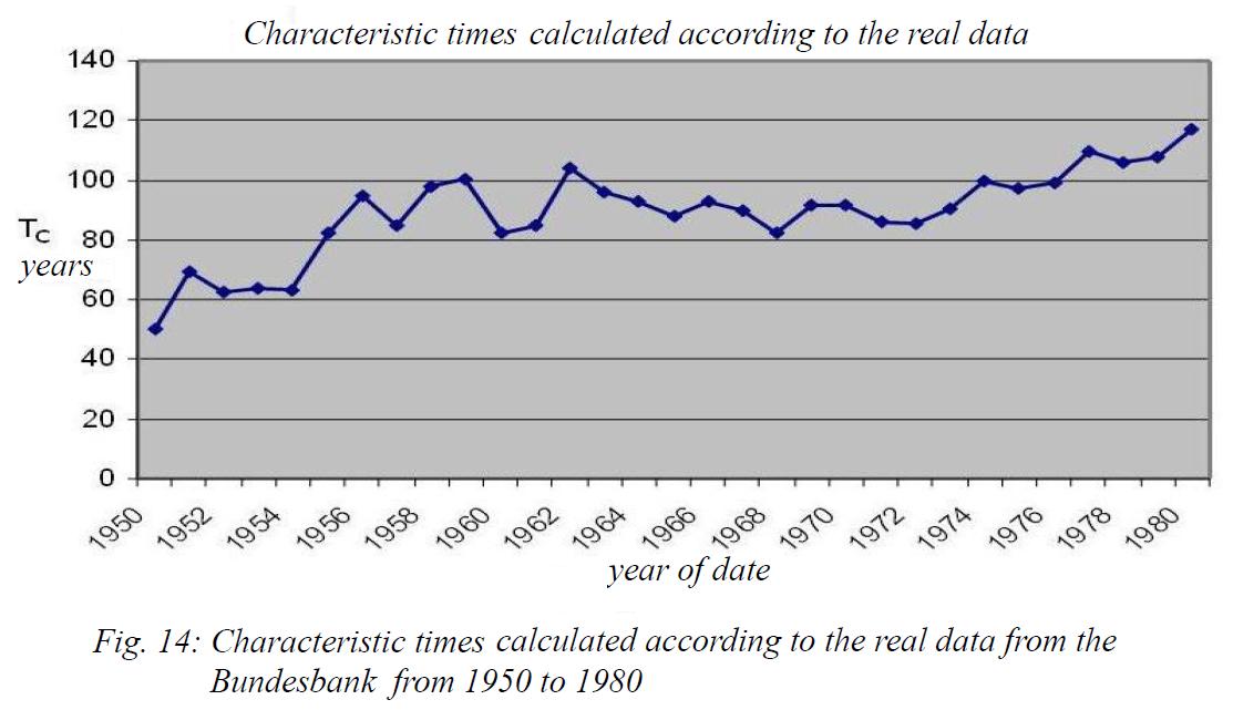
We can see
these characteristic values in the following figures, calculated according to
the official figures of the FRG: In the beginning the characteristic time![]() represents the
critical period
represents the
critical period![]() given by the compound
interest rule of thumb next chapter. For the range of initial conditions
given by the compound
interest rule of thumb next chapter. For the range of initial conditions![]() we get about
we get about ![]() years.
years.
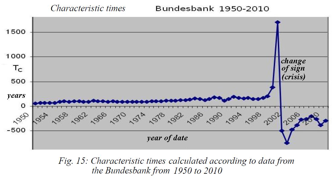
But after
that![]() grows strongly
and ultimately turns sharply to negative values. This inflection point is given
by the year 2000. For the growth path of the economy thus the parameter
grows strongly
and ultimately turns sharply to negative values. This inflection point is given
by the year 2000. For the growth path of the economy thus the parameter
![]()
is crucial. It must be kept negative to stay in
the growth-regime of the![]() and thus does not
enter into the realm of the down-sloping
and thus does not
enter into the realm of the down-sloping ![]() .
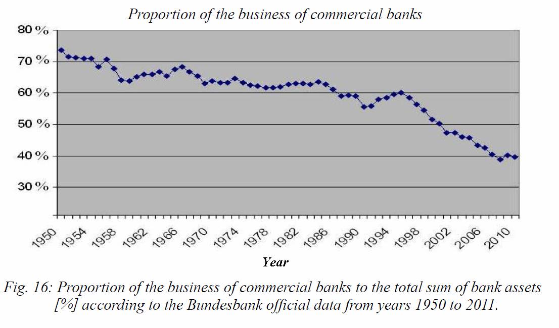
Since 2001, but this value is positive in the FRG. The share of domestic
lending business has declined since 1950 by almost 73% to less than 40%. To
assess the growth parameters we reflect again on the importance of individual
variables.
.
Since 2001, but this value is positive in the FRG. The share of domestic
lending business has declined since 1950 by almost 73% to less than 40%. To
assess the growth parameters we reflect again on the importance of individual
variables.
It is the condition
![]() (19.10)
(19.10)
to comply, which in turn gives the conditions
for![]() greater or less
zero:
greater or less
zero:
![]() :
:
![]() (19.11)
(19.11)
![]() :
:
![]() (19.12)
(19.12)
As we see it is in each of the four cases in
turn critical if the relative share of investment in the real economy![]() is larger or less
than 50%, which is the same as
is larger or less
than 50%, which is the same as![]() is greater than
or less than zero.
is greater than
or less than zero.
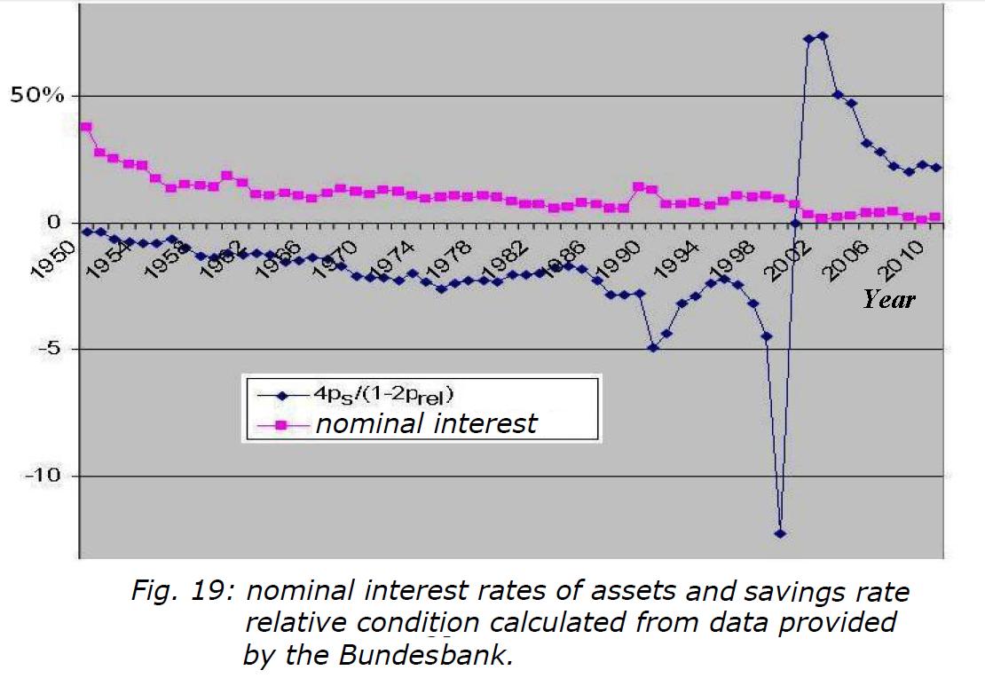
In the next
graph we can see, calculated according to official figures from the Bundesbank,
the growth frequency![]() (scaled40 by the factor 50) and the share of
real investment
(scaled40 by the factor 50) and the share of
real investment![]() (scaled by 4).
One can clearly see how the crisis situation since 2000 is associated with the
decline of real credit share below 50% and also the drop in growth rate below
zero.
(scaled by 4).
One can clearly see how the crisis situation since 2000 is associated with the
decline of real credit share below 50% and also the drop in growth rate below
zero.

Potential strategy for how you can still stay on a positive growth path, we must therefore continue to consider the four different cases F1 to F4:
![]() (F1)
(F1)
![]() (19.13)
(19.13)
![]() (F2)
(F2)
![]() (19.14)
(19.14)
![]() (F3)
(F3)
![]() (19.15)
(19.15)
![]() (F4)
(F4)
![]() (19.16)
(19.16)
Until 2000 the case F2 was present in
the FRG. We see here on the official figures, the FRG typical high savings
rate. The relevant limit value![]() is
maintained until the year 2000.
is
maintained until the year 2000.
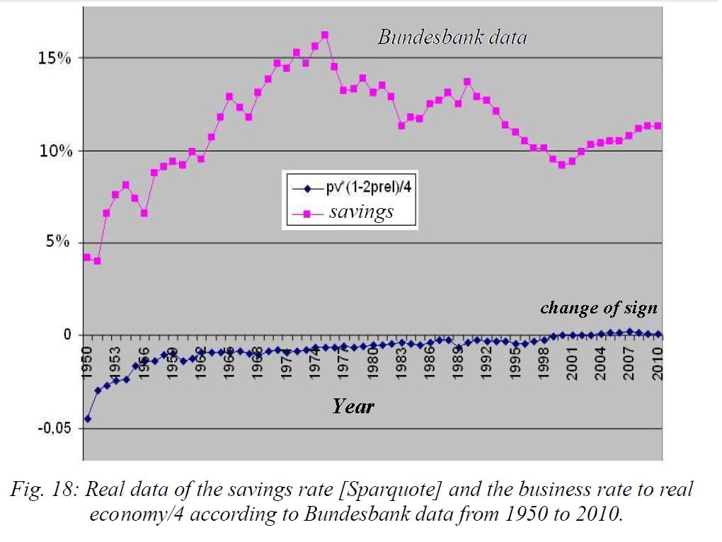
Afterwards,
however, the value of![]() changes its sign,
because since then the value of the share of investment to the real economy
fell below 50%.
changes its sign,
because since then the value of the share of investment to the real economy
fell below 50%.
Thus, we switch to F1 case with the condition![]() for the growth
path. Currently
for the growth
path. Currently![]() is only about 40%
at a nominal interest rate of less than 2%, and thus
is only about 40%
at a nominal interest rate of less than 2%, and thus![]() would have to
apply. This means that the savings rate would have to be less than <0.1%,
thus best negative, in order to remain on a growth path. Alternatively, would
also be a negative nominal interest rate
would have to
apply. This means that the savings rate would have to be less than <0.1%,
thus best negative, in order to remain on a growth path. Alternatively, would
also be a negative nominal interest rate![]() of bank assets imaginable. One possibility would then be the case F3.
That would mean that with a high proportion of investment banking, with a
savings rate of
of bank assets imaginable. One possibility would then be the case F3.
That would mean that with a high proportion of investment banking, with a
savings rate of
![]() , e.g.
, e.g. ![]() ,
,
the growth condition would also continue to be
met with a positive savings rate.
Remains finally the case F4: So likewise, a negative nominal interest
rates![]() of assets, but at
reduced investment share, and a savings rate of condition of
of assets, but at
reduced investment share, and a savings rate of condition of
![]() , e.g.
, e.g.![]() .
.
The last example also shows the growth
condition, that meets the growth path only with negative savings rate. One can
clearly see the importance of the relative ratio of investment in the real
economy![]() in the next
graphic. Because of positive nominal interest rate always
in the next
graphic. Because of positive nominal interest rate always![]() is to demand.
is to demand.
The latter
value does, however, with the fall of![]() below
the 50% level, and thus the preponderance of bank equity business, a sign
change. So unattainable with the FRG typical high savings rate is above
condition. To return to growth path thus the possibilities are limited. The
result would call into question, to reduce the savings rate to well below zero.
below
the 50% level, and thus the preponderance of bank equity business, a sign
change. So unattainable with the FRG typical high savings rate is above
condition. To return to growth path thus the possibilities are limited. The
result would call into question, to reduce the savings rate to well below zero.