31 Analysis of Inflation

The official inflation levels are determined by the statistical offices by calculating the yearly percentage change in the value (CPI) of a product basket. These values are a more or less good approximation to the actual inflation, depending on the chosen basket and the algorithm for calculation. Deflation is in accordance with the case when the cart gets cheaper. However, due to the nature of the investigation depending on the selected basket, that will and must also change over time necessarily, as the consumer desires and habits change, as well as with technological changes and social change does apply, this number is always approximately. To make matters worse, these values are increasingly effected by the method of Hedonic⁶⁵ regression. Such processes lead to reduced rates of inflation and higher official GDP growth. Depending on the scope of hedonic regression. effects are enormous. Correctly, the government should publish nominal raw data in addition to the institute's hedonised figures, as for ecomomic growth modeling just the raw data matter. They do this however rarely, and also the exact method of calculation of the specific shopping carts and hedonizing rates remain practically in the unknown.

Inflation but is an intrinsic effect of all economies and can be derived from the sources and sinks and thus calculated also theoretically. For this we look at our source equation in more detail. We differentiate the equation with respect to the time t and then sort by price level to

    (31.1)

which we also can write in short as

    (31.2).

We already see here the effect we can also see clearly when looking at the statistically calculated rate of inflation: the price level is modulated with the pre-factor V. As the price level is dependent on the temporal change of K and V clearly, but in particularly is important the last term in the above equation, because there only is the sign negative and H in the inverse square is received. This means that the critical trading-term is

    (31.3)

and thus can have a significant impact on price levels, because both can completely reverse the trend, and by reason of its reciprocal value, as well let it “explode”. It is further given by a simple transformation:

    (31.4)

reflecting the fundamental importance of the trading volume for the pricing level. The inflation rate is now a relative value, namely the normalized price change on the price level:

    (31.5)

Resorting to the characters and introducing I for Inflation makes up to:

    (31.6)

This fundamental equation, we should consider briefly. Thusrepresents the classically known fact that the inflation rate is mainly determined by the ratio of monetary velocity to GDP. Furthermore, the factor is still effective. This modulates the rate of inflation with the development of the stock of capital. Thus, the inflation rate is higher if the price of capitalincreases, which makes sense. It gets however smaller, when a lot of capital K, multiplied by the relative growth of H plus V, is available. Because the last term generates a cash inflow to GDP, which reduces the need for capital and thus the price of capital, and thus also for produced and traded goods. From this equation we can now also create an ODE for what is the fundamentally important trade volume, by solving the inflation differential equation (30.6) for H:

    (31.7)

For the case distinction we can now define partial solutions by assuming first of all, that the unstable phase, namely the validity of the quadratic term H has not been reached yet. Disregarding the quadratic term of H integrates the expression slightly. The result is analytically the quasi-stable solution:

    (31.8)

The quotientis the growth rate of GDP, as it usually is communicated, and the constant of integrationis the trading volume at the start of development. This means at the beginning of an economy that economic growth goes hand in hand with the trading volume actually increasing exponentially at first. The time t is counted here from the zero point of the national economy or the first point of calculation. If after the saturation phase crisis occurs , the quadratic term H gets increasingly important and takes the lead. By deleting the then much smaller previous terms we can integrate the last term separately, and thus obtain the solution of the quasi-unstable state:

    (30.9)

In the ultimate crisis, but only there, the price increase, which is usually more trade promoting, becomes then a devastating effect because of its steep slope: it leads to a trade decline, which is because of the inverse square term but now a desastrous effect :

    (31.10)

Namelythen gets sharply positive, as isnow. The result is a tighter inflation, and thus threatens to refuse additional trade, making the term growing more fast. Also, a simultaneous decline of GDP Y cannot stop this, as Y enters only linearly. The constantis the time from the start of the downturn. For this time is approximateand thus we get for the trade volume on the crisis path:

    (31.11)

Here we only have to add an expression for. For this we exploit the fact that now the price level before the crisis is fully determined by

    (31.12).

It is given by a longer⁶⁶ calculation the change in the price level to:

    with

And   

(31.13)

This expression we can now invest in the above formula of H(t) in order to calculate the volume of trade in normal times. It is therefore the approximate formula

    (31.14)

The normal rate of inflation in turn is then only calculating⁶⁷ analytically:

(31.15)

Thus, inflation in normal times should be determined by this calculation. This expression can be simplified somewhat, such as the last term vanishes forslowly variable savings rates. Further simplification can be assumed also that the savings rate is significantly less than 1, and thus is again approximately 1. This results in:

    (31.16)

Even further, we can assume from experience that the second derivative of growthis very small, because the growth of the growth is almost very low. But certainly this is not valid for the compound interest, which stems⁶⁸ from the ever growing total capital stock. For the analytical core inflation, we can therefore write:

    (31.17)

Or in terms of slip rates of growth

    (31.18)

still being received, that the percentage of compound interest is about . The actual inflation rate is now up to a constant factor c, which we had also to take into account with the trading volume as an undetermined constant, which provides:

    (31.19)

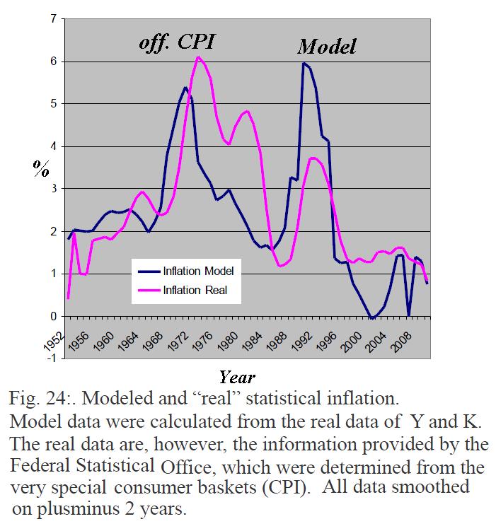
We can determine c to, and thus we get Fig. 25 for the approximation (31.17):