43 The Predator-Prey Symmetry
Real solution will break the latest, when the
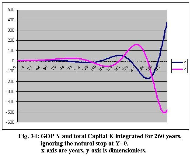
GDP has fallen to zero. To examine the formal structure of the linear system of
equations, we but can simply continue to run the equations beyond the endpoint![]() . In the
following figure, we see the resulting effect: The
solutions for K and Y will oscillate somehow out of phase around
the zero line. It does, however, increase the maximum amplitude in time
exponentially.
. In the
following figure, we see the resulting effect: The
solutions for K and Y will oscillate somehow out of phase around
the zero line. It does, however, increase the maximum amplitude in time
exponentially.
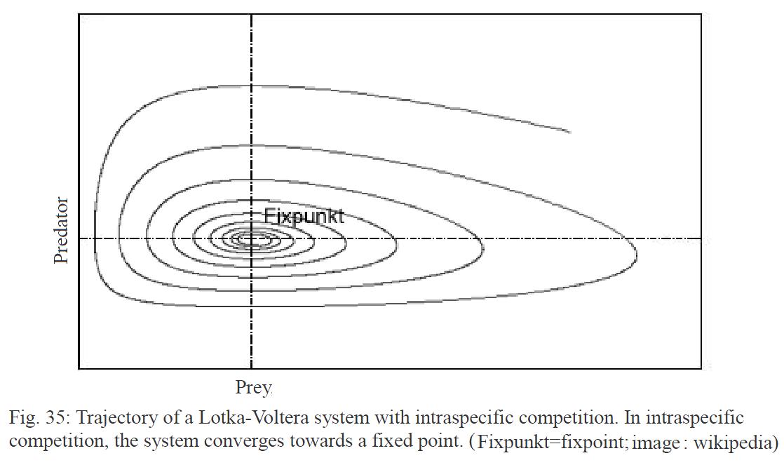
Such solutions are typically found in so-called "predator-prey" models (PPM), derived from theoretical biology. The most prominent PPM is the Lotka-Volterra model, which was already established in the 19th-century, to explain the dynamics of populations of the animal kingdom.The Lotka-Volterra equations are::
![]()
![]() (43.1)
(43.1)
 Now the basic system of a national economy is of a similar structure:
![]()
![]() (43.2)
(43.2)
for the “meeting” of capital and GDP
has different effects on GDP and capital stock. In particular![]() is the result of
the encounter
is the result of
the encounter
![]() . Similarly,
however, are savings
. Similarly,
however, are savings
![]() because it
depends on an appropriate encounter
because it
depends on an appropriate encounter![]() of
the two. Thus in principle
we can
write:
of
the two. Thus in principle
we can
write:
![]()
![]() (43.4)
(43.4)
The term![]() we
have just inserted in order to demonstrate the same type of structure here. The
difference lies in the very different structure of the reproduction rates of
the two populations. The first term of the second equation, we can also replace
by net exports, which would ideally be zero, but often is not:
we
have just inserted in order to demonstrate the same type of structure here. The
difference lies in the very different structure of the reproduction rates of
the two populations. The first term of the second equation, we can also replace
by net exports, which would ideally be zero, but often is not:
![]()
![]() (43.5)
(43.5)
The different problem is
ergo, that the growth rates![]() and
and
![]() are not fed back to each other. This does not result
in a converging, but a as we will see, in divergent behavior.
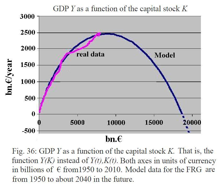
We thus want to investigate this further. Now you can also simply indicate that
GDP is a function of capital, so instead of the two functions Y(t) and K(t), we can now draw the
derived one function Y(K). So we change our reference room, to come to a
simpler but more meaningful representation. For this, we just have to plot the
real data of Y and K and the basis model data as well to show. At
first glance, this appears to be a function as a parable, and in fact they can
be approximated with a high confidence level for the FRG with the regression
are not fed back to each other. This does not result
in a converging, but a as we will see, in divergent behavior.
We thus want to investigate this further. Now you can also simply indicate that
GDP is a function of capital, so instead of the two functions Y(t) and K(t), we can now draw the
derived one function Y(K). So we change our reference room, to come to a
simpler but more meaningful representation. For this, we just have to plot the
real data of Y and K and the basis model data as well to show. At
first glance, this appears to be a function as a parable, and in fact they can
be approximated with a high confidence level for the FRG with the regression
![]() (43.6).
(43.6).
This is a practical rule of thumb to us, from which we get the GDP Y to be expected with a capital stock of K in the FRG.
The rule of thumb
![]() (43.7)
(43.7)
can be determined and used for each country N, without large external net premiums, slightly. The coefficients are sorted according to their meaning, here for the FRG:
![]() GDP-Offset
(
GDP-Offset
(![]() )
)
![]() Average
Capital Efficiency
Average
Capital Efficiency
![]() Repressional Capital Coefficient
Repressional Capital Coefficient
The constant![]() describes
in principle the GDP at the beginning of the census, compounded from
describes
in principle the GDP at the beginning of the census, compounded from![]() with inflation.
We already know the constant
with inflation.
We already know the constant![]() which is nothing
more than the average capital efficiency, which was for the FRG nearly 52%. So
in the long term one half of capital goes into the real economy, the other half
into the building up of the capital. The constant
which is nothing
more than the average capital efficiency, which was for the FRG nearly 52%. So
in the long term one half of capital goes into the real economy, the other half
into the building up of the capital. The constant
![]() now describes the negative feedback by the with
time increasing amount of return on capital as the pressure on the GDP
ultimately resulting from the compound interest. We call it, because of its low
absolute, but due to the entrance to the square of the capital increasing
weight, as the Capital Repression Coefficients
now describes the negative feedback by the with
time increasing amount of return on capital as the pressure on the GDP
ultimately resulting from the compound interest. We call it, because of its low
absolute, but due to the entrance to the square of the capital increasing
weight, as the Capital Repression Coefficients
![]() with
its unit is
with
its unit is![]() .
From the regression equation
.
From the regression equation
![]() (43.8)
(43.8)
the solution is for![]() given
by
given
by
![]() (43.9)
(43.9)
and with the values for the FRG we get![]() bn. €/year, the latter of which is the maximum
positive value of capital stock, while for the GDP to the value zero is
depressed. The maximum of the development is given by
bn. €/year, the latter of which is the maximum
positive value of capital stock, while for the GDP to the value zero is
depressed. The maximum of the development is given by
![]() at
at ![]() (43.10)
(43.10)
with ![]() Billion
€ for the FRG. This is the maximum value of the capital raising ability
of the
Federal Republic until the turn of development.
Especially the final value
Billion
€ for the FRG. This is the maximum value of the capital raising ability
of the
Federal Republic until the turn of development.
Especially the final value![]() is in the extent
of theoretical nature, as we would assume that until finite decline all market
participants would behave unaffected by the development. At the latest after
exceeding the maximum
is in the extent
of theoretical nature, as we would assume that until finite decline all market
participants would behave unaffected by the development. At the latest after
exceeding the maximum
![]() but this is
increasingly unlikely, and the artificial interventions in the monetary and
economic system are increasing. This leads to the relevant variables
but this is
increasingly unlikely, and the artificial interventions in the monetary and
economic system are increasing. This leads to the relevant variables![]() and
and![]() getting more and
more important in the basic equations .
getting more and
more important in the basic equations .