47 Rotational-Stretching-Symmetry

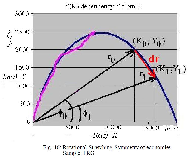
If we want to transfer the position vector from the Y-K-space currently used into the usual Y,K-t-space at the time to the time , then we can achieve this with the help of a rotational expansion. The rotational extension symmetry is the same symmetry, as occurs in the multiplication of imaginary numbers:

    (47.1)

Our position vectors are as shown above, just

and     (47.2),

where we have set Y in the imaginary direction, ie in general

    (47.3)

for the position vector. The expressionis often associated with the function

    (47.4)

and abbreviated. It is now apparent manner:

    (47.5)

or

    (47.6)

with the implicit Logspiral-representation . The effect of rotation and expansion is evidently composed of inflation or Pricingand trading gain. How true that is easily verified

    (47.7)

and

    (47.8).

We see here already thatmoves on its own axis of GDP, whileaffects the GDP and capital axis equally. Because inflation affects both the capital and the value of GDP both measured in money. The implicit representation

results in and .

Inserting brings:

    (47.9)

The effect of the helical symmetry is that now enters the commercial growth in the real and imaginary parts as well.

The dynamics of economic development thus corresponds allways to a rotation and expansion, so that a change in trade is always accompanied by a price change due.

The division of two complex numbers is given by, and thus can⁸⁸ be written:

    (47.10)

Because ofandatit follows:

    (47.11)

and     (47.12)

This implicit representation we have to convert into a suitable explicit time dependence. Forresults in the meantime:

    (47.13)

and further to resolve complex fortakes after some merging:

    (47.14)

with the abbreviations:

,,,

,,  and     (47.15).

And in accordance with this the inflation or price-formation is

(47.16).

Then there is the transformation back to the usual time dimension. For this we assume the mathematical relationship

(47.17)

The angular velocitywe can determine by use of the start and end time of the model economics. Because the angle was 90 degrees = at the beginning, and 0 at the end in our vector space of Y(K)-representation. Therefore, one may write as we start counting at:

und (47.18)

This isthe time when the GDP dropped to zero in basis theory. With

and (47.19)

one can now determine in principle the behavior of price formation and trading volume in the usual time dimension.