48 Commutator Symmetry

We make here a mathematical bond in quantum mechanics. The term of the commutator comes from a household context. Among the commonly used in everyday life numbers are numbers that are subject to some simple group symmetries. One such group is the commutativity properties, or rewrite it as. This symmetrie can be written abbreviated as

    (48.1).

The brackets [] is called the "commutator", and the right side of the equation "commutator-residue". This residue must be but not zero in the general case. If the commutator-residue is zero, it is called Abel's numbers, if it is not equal to zero, whereas called non-Abelian numbers. Elementary particles are represented in particular by such non-Abelian numbers. The mathematical "trick" here is that those numbers are represented by so-called "operators". Operators are, as the name suggests, some mathematical gadgets that do anything when applied to other numbers, say, in the case of differential operators that make a differenciation. The commutator-residue if it is not zero.

Let, therefore, look us again on the derivation of the previous one. When considering the quantity equation in the SMF, we have the relationship

to derive the average monetary velocity. This structure enables us to sort something:

or

or

    (48.2).

We can now write in the so called operator notation:

    (48.3)

with the operators

   and        (48.4).

From quantum mechanics we know the simple coherences of this elementary symmetries

    (48.5)

known about the properties of atoms and their constituents do. This meant that the KV-operator defined here is applied to Y and so that KV product is produced. Thus we get:

    (48.6)

The commutator-residue should we expect equal zero as in the economy we use always finite abelian numbers. So either, which almost never happens, or specify:

   or        (48.7)

Now isprecisely the nominal return on capital (and derived from that also namelyor):

    (48.8)

what gives the desired results in relation to the average return on all assets of an economy. The interest rate we can now compare with the supply-demand estimate at the beginning of the second part of the book.
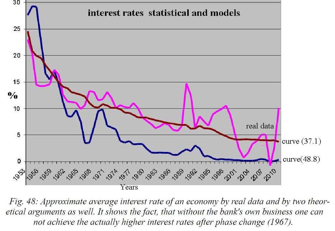
In the next graph we see the result. The real change in the total nominal capital stock, is roughly equivalent to the nominal interest rate on all assets. The curve (37.1) with) comes very close. This corresponds to the fact that in the underlying function, also for the product money, there is an effective supply-demand ratio.
The curve (:48.8) on the other hand, goes faster to zero than the real numbers. The reason for this lies in our simplified derivation in which onlyoccurs but not. The investment business is therefore not included. Therefore (48.8), follows the curve of the real numbers only up to the region of the phase change in 1967, and then falls off more quickly, since without the bank's own business can not be achieved then actually higher interest rates. Before phase change the interest rates would have been even higher, due to the same effect in the other direction, as then loans to the real economy would have been the better choice.