11 Monetary Inflation Correction and Calibration

So our model is basically calculated in dimensionless "points". Because currency is purely nominal, whether dollars, rubles, euros or pounds, or points, it makes no difference. Except the multiplication by a conversion factor c. To convert the values calculated in points in latest monetary data, it is necessary to determine this conversion factor. Here are some considerations necessary. Trivially, we would begin:

and    (11.1)

with the conversion constants

   (11.2)

This leads to no useful result, because the time-dependent inflation is absent, and the final value is nominal too small then (the relative numbers but remain unaffected). The GDP Y is fundamentally affected by its growth, but additionally there is the nominal effect of inflationtoo, as GDP is calculated in units of currency. This just looks natural on the capital stock K, which is in addition but in contrast to GDP, effected by the interest rate. This last effect²⁵ is of course fully contained in our computation. What makes inflation so mathematically, is to convert the conversion constantinto a time-dependent variable. Thus the scores of Y and K have to be converted into monetary units by defining and computing the additional effect of inflation.

There are several possibilities to do this. The most elegant method would be now, of course, with the inflation calculated analytically. This is indeed possible but as it is far from trivial, it will been explained later in this book. The second possibility would be to use the statistical official rate of inflation , which is derived from the evaluation of a shopping basket. However, among those already described, and unfortunately very serious, limitations which can not give good results. Until we can calculate analytically the actual inflation rate, so we must be content with the simplest possible approximations. There are again several possibilities. First, trivially, but now with a time dependence c:

and    (11.3)

and with the conversion functions

and      ?? (11.4).

Such an approach is ruled out, however, because it is "through the chest from behind through the eye". For one then incorporates into the model the real values, where they should not be for model consistency. Better, and model-theoretically justified, is a simple linear approximation. The ratio V of points is determined by the total nominal GDP in currency and capital stock at the beginning

    (11.5)

and at the end

    (11.6)

of the integration, and one linearly interpolates the intermediate values:

    (11.7)

The model values in currency units are obtained in this case then as

    (11.8 a)

and

    (11.8 b)

which are now functions with the same linear conversion factor correctly are provided both to Y and K. In the above plot we see the two functions on the approach (11.4) and the approach to (11.8) of the correction function V in comparison.

Why is the ratioapproximately linear growing at all, as one should expect naive that inflation and capital cuts out in the quotient? The reason is that capital is not degraded, but very probably the GDP, which is very well subject to depreciation. But now what is the reason for the relative linearity in the increase in capital ratio? Let us consider again our basic equation simplified, and that without integrating them. Even then you will already recognize many basic properties and relationships. We therefore take simply the ratio of capital productivity from our formula (3.3):

      (11.9)

Now the coefficient of capital productivity is not identical to the rate of inflation, but it is closely related to it. For if the growth of capital does not equal to the GDP growth, inflation or deflation is then to be expected. Therefore, where a(t) is our exponential prefactor, rules:

    (11.10)

Let us now examine the official inflation rate, which was determined by the Federal Statistical Office, in comparison to the capital productivity, where the constant factorwas chosen: In Figure 8 you can see the amazing parallel course. An improved interpolation is therefore possible with an exponential form

    (11.11).

For the FRG a numerical solution results in:

    (11.12)

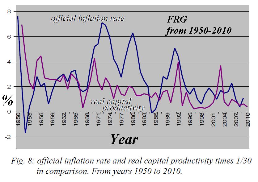
Why do we take for calibration not the official inflation rate? It is not possible because the official inflation rate is only a relatively crude statistical approach to a not yet well understood problem. The official inflation basket varies greatly, and is in the long-term average of about 2.5%. The weightings of the basket of products, that are different for each consumer class and also different in their underlying assumptions, are to be questioned even more critical. As the official inflation rates²⁶ and the subjective impression of the citizen from official numbers differ, recently in the FRG was also the notion of “perceived inflation” introduced, which is determined from other criteria and is significantly higher.

As a final gauge, we can look to us therefore the ratiowhich occurs, if we determined it from the official "average-consumer" basket inflation data. First one notices, that the official average gradient of 2.5% is too low. Therefore it makes the unavoidable impression that the inflation rate would be systematically underestimated. Only when we introduce a constant factor²⁷ of 1.8 we approach the real values close enough.